Lecture 2
Image Classification
What a machine sees -> (Red, Green, Blue) intensity (0~255)
A image is just a 2-D matrix of integers between[0, 255]
600 x 800 x 3 (RGB) -> tensor
Challenges
viewpoint variation + background clutter + illumination + Occlusion + Deformation + intra class variation
Machine learning : Data-Driven approach
- Collect a dataset of images and labels
- Use a machine learning algorithm to train a classifier
- use the classifier to predict unseen images
Nearest Neighbor
def train(self, images, labels):
    # simply remembers all the training data
    self.images = images
    self.labels = labels

def predict(self, test_image):
    # assume that each image is vectorized to 1D
    min_dist = sys.maxsize  # maximum integer in python
    min_index = -1  # 초기값 설정
    for i in range(self.images.shape[0]):
        dist = np.sum(np.abs(self.images[i, :] - test_image))
        if dist < min_dist:
            min_dist = dist
            min_index = i

    return self.labels[min_index]
With N training examples,
-For training O(1)
-For prediction O(N)
Parametric Approach
instead of memorizing all training examples,
think of a function f that maps the input (image x) to the label scores ( class y)
image x -> f(x) -> class
image x 에 weights or parameters W 를 곱해주고 그 값
어느 픽셀의 가중치가 커야 어느 class 에 점수가 오르는지
각 이미지에 각 class 의 weight 를 곱해준다.
f(x,W) 10x1 = 10 x 3072 (W) 3072 X 1 (x) + B
B 만약 데이터 셋에 고양이 강아지가 많다면 맞추기 위해 다른 고양이 강아지만 고른다. 테스트 데이터셋에 고양이 강아지가 나올거라고 생각
데이터랑 상관없이 정해지는 B 10 x 1
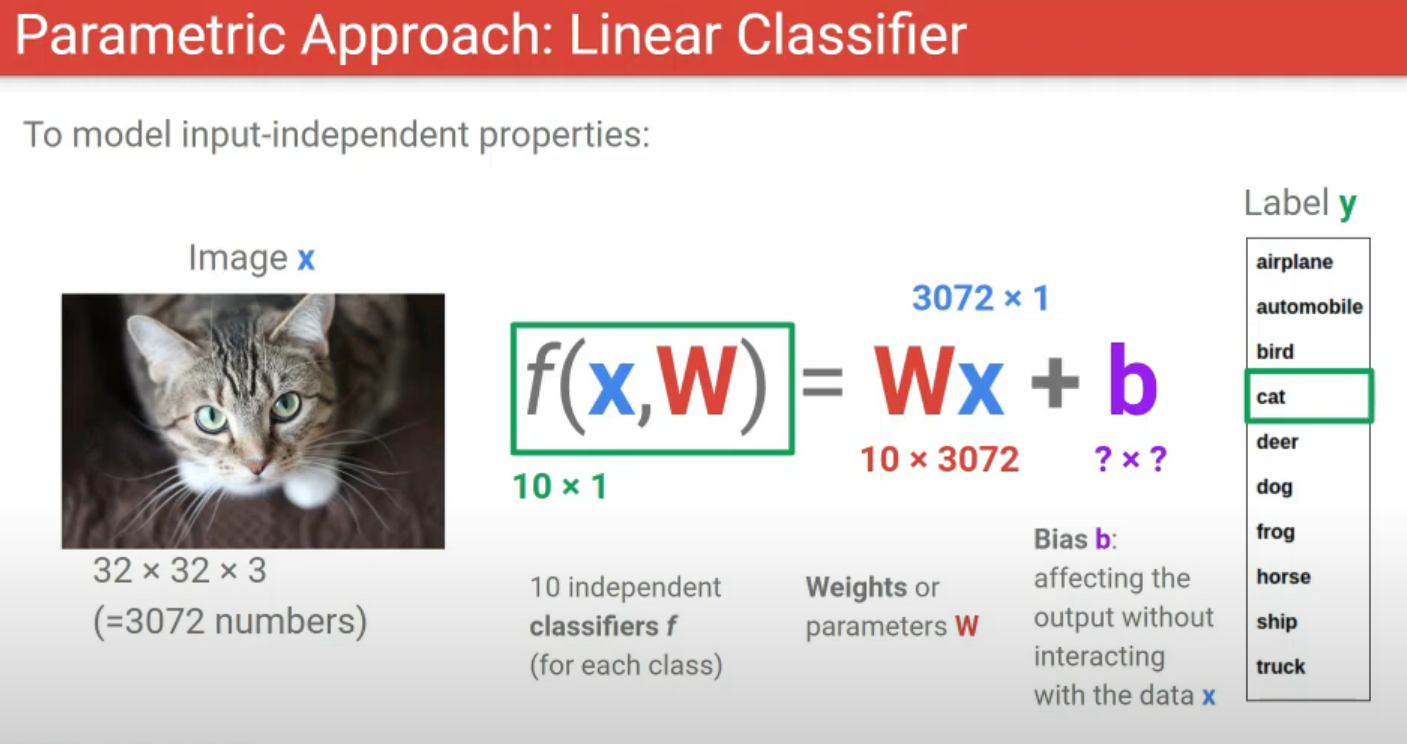
parametric approach linear classifier
nearest neighbor 이랑 똑같지. 근데 데이터를 외운 것과 데이터를 통해 배운다.